Example 2: Exploring your data graphically.
example2.RmdBarplots, boxplots or normality plots are displayed according to the nature of described variable. These plots are useful to explore visually whether a continuous variable follows a normal distribution or to identify possible outliers or rare categories, etc.
Step 1. Install the package
Install compareGroups package from CRAN
and then load it by typing:
install.packages("compareGroups")
library(compareGroups)Setp 3. Computations
First use compareGroups function to store all values
used to perform plots afterwards.
res <- compareGroups(year ~ . , data = regicor)You can use varinfo
function to recover the original name of variables (not labels which are
displayed in the results).
varinfo(res)
--- Analyzed variable names ----

   Orig varname Shown varname
1  year         Recruitment year
2  id           Individual id
3  age          Age
4  sex          Sex
5  smoker       Smoking status
6  sbp          Systolic blood pressure
7  dbp          Diastolic blood pressure
8  histhtn      History of hypertension
9  txhtn        Hypertension treatment
10 chol         Total cholesterol
11 hdl          HDL cholesterol
12 triglyc      Triglycerides
13 ldl          LDL cholesterol
14 histchol     History of hyperchol.
15 txchol       Cholesterol treatment
16 height       Height (cm)
17 weight       Weight (Kg)
18 bmi          Body mass index
19 phyact       Physical activity (Kcal/week)
20 pcs          Physical component
21 mcs          Mental component
22 cv           Cardiovascular event
23 tocv         Days to cardiovascular event or end of follow-up
24 death        Overall death
25 todeath      Days to overall death or end of follow-up
Step 4. Perform plots
by using the plot method which takes the results created
by compareGroups function.
Inside “[” brackets you can select which variable to plot. And,
indicating bivar=TRUE a bivariate plot is performed,
i.e. stratifying by groups.
- For categorical variables a barplot is performed, stratifying by groups (right plot) or not (left plot):
plot(res['sex'])
plot(res['sex'], bivar=TRUE)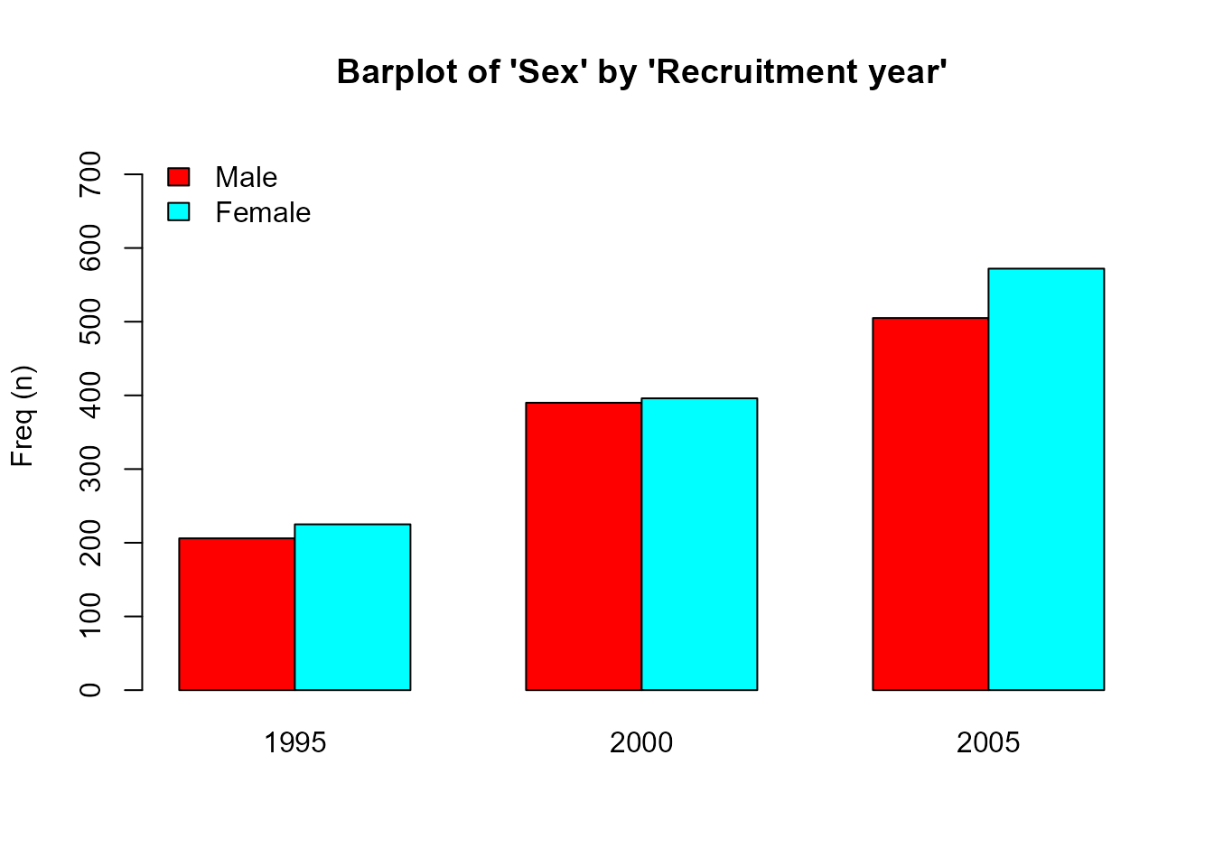
- For continuous variables boxplots or normality plots are performed depending whether groups are considered or not, respectively.
plot(res['bmi'])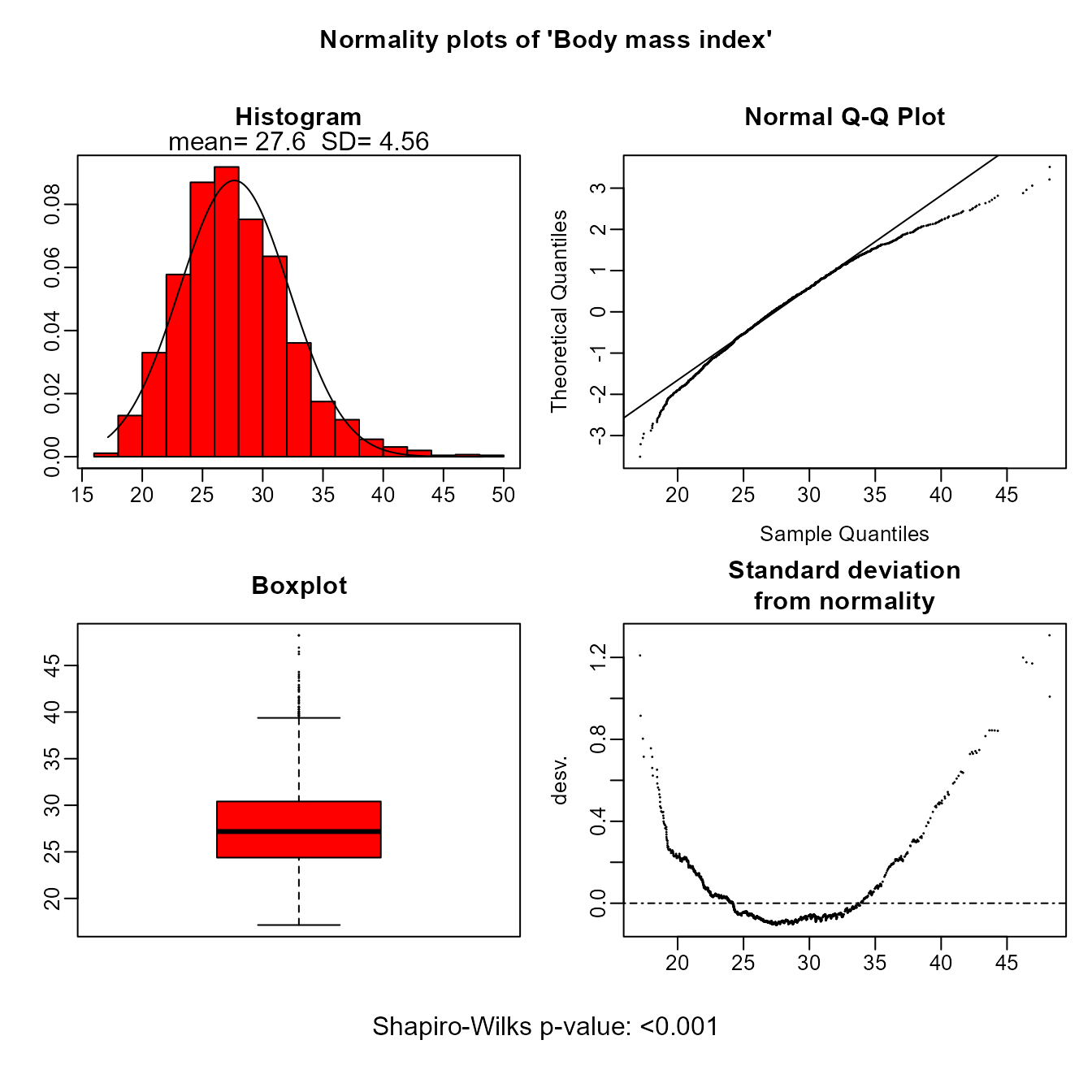
plot(res['bmi'],bivar=TRUE)