package to create descriptive tables
Overview
compareGroups is an R package available on CRAN which performs descriptive tables displaying means, standard deviation, quantiles or frequencies of several variables. Also, p-value to test equality between groups is computed using the appropiate test.
With a very simple code, nice, compact and ready-to-publish descriptives table are displayed on R console. They can also be exported to different formats, such as Word, Excel, PDF or inserted in a R-Sweave or R-markdown document.
You will find an extensive manual describing all compareGropus capabilities with real examples in the vignette.
Also, compareGroups package has been published in Journal of Statistical Software [Subirana et al, 2014] (https://www.jstatsoft.org/v57/i12/).
Who we are

compareGroups is developed and maintained by Isaac Subirana, Hector Sanz, Joan Vila and collaborators at the cardiovascular epidemiology research unit (URLEC), located at Barcelona Biomedical Research Park (PRBB) .
![]()
As the driving force behind the REGICOR study, URLEC has extensive experience in statistical epidemiology, and is a national reference centre for research into cardiovascular diseases and their risk factors.
Gets started
Install the package from CRAN
or the lattest version from Github
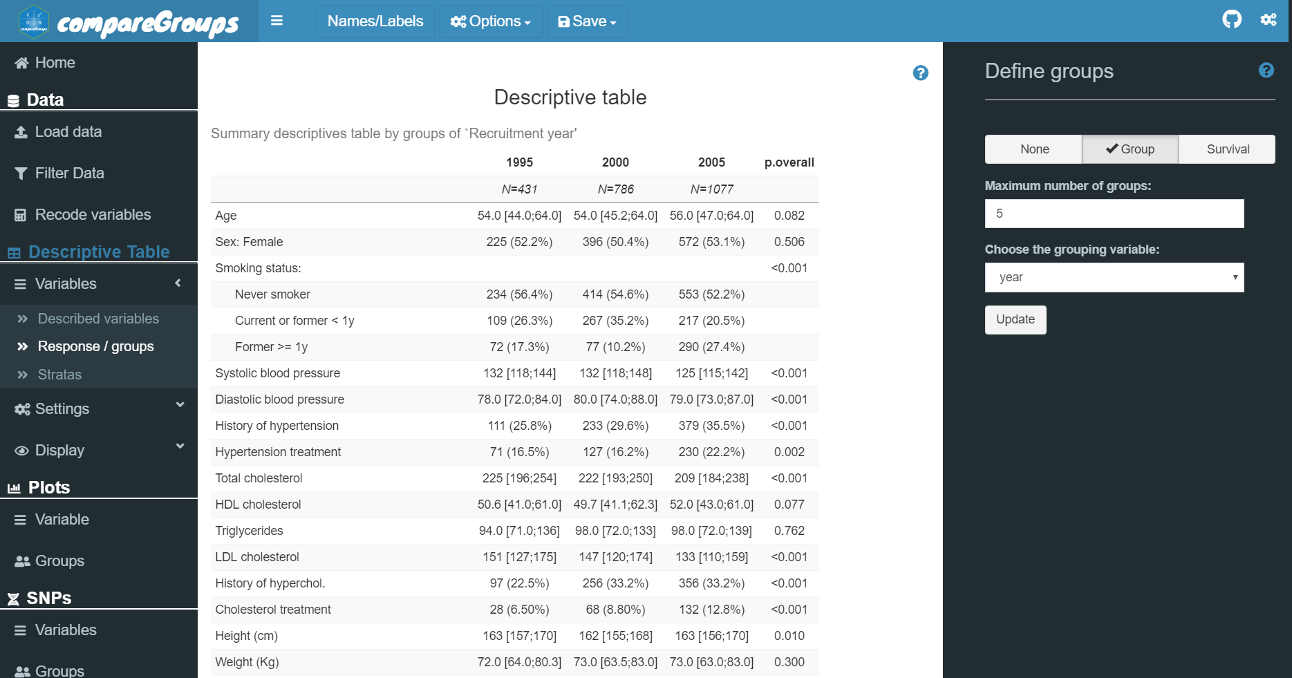
Building the descriptive table
library(compareGroups)

data(regicor)

tab <- descrTable(year ~ . -id , regicor, hide.no = "no",
                  method=c(triglyc=2, tocv=2, todeath=2), sd.type = 3)

export2md(tab, header.background = "black", header.color = "white",
caption = "Summary by intervention group")| 1995 | 2000 | 2005 | p.overall | |
|---|---|---|---|---|
| N=431 | N=786 | N=1077 | ||
| Age | 54.1±11.7 | 54.3±11.2 | 55.3±10.6 | 0.079 |
| Sex: | 0.506 | |||
| Male | 206 (47.8%) | 390 (49.6%) | 505 (46.9%) | |
| Female | 225 (52.2%) | 396 (50.4%) | 572 (53.1%) | |
| Smoking status: | <0.001 | |||
| Never smoker | 234 (56.4%) | 414 (54.6%) | 553 (52.2%) | |
| Current or former < 1y | 109 (26.3%) | 267 (35.2%) | 217 (20.5%) | |
| Former >= 1y | 72 (17.3%) | 77 (10.2%) | 290 (27.4%) | |
| Systolic blood pressure | 133±19.2 | 133±21.3 | 129±19.8 | <0.001 |
| Diastolic blood pressure | 77.0±10.5 | 80.8±10.3 | 79.9±10.6 | <0.001 |
| History of hypertension | 111 (25.8%) | 233 (29.6%) | 379 (35.5%) | <0.001 |
| Hypertension treatment | 71 (16.5%) | 127 (16.2%) | 230 (22.2%) | 0.002 |
| Total cholesterol | 225±43.1 | 224±44.4 | 213±45.9 | <0.001 |
| HDL cholesterol | 51.9±14.5 | 52.3±15.6 | 53.2±14.2 | 0.198 |
| Triglycerides | 94.0 [71.0;136] | 98.0 [72.0;133] | 98.0 [72.0;139] | 0.762 |
| LDL cholesterol | 152±38.4 | 149±38.6 | 136±39.7 | <0.001 |
| History of hyperchol. | 97 (22.5%) | 256 (33.2%) | 356 (33.2%) | <0.001 |
| Cholesterol treatment | 28 (6.50%) | 68 (8.80%) | 132 (12.8%) | <0.001 |
| Height (cm) | 163±9.21 | 162±9.39 | 163±9.05 | 0.004 |
| Weight (Kg) | 72.3±12.6 | 73.8±14.0 | 73.6±13.9 | 0.120 |
| Body mass index | 27.0±4.15 | 28.1±4.62 | 27.6±4.63 | <0.001 |
| Physical activity (Kcal/week) | 491±419 | 422±377 | 351±378 | <0.001 |
| Physical component | 49.3±8.08 | 49.0±9.63 | 50.1±8.91 | 0.037 |
| Mental component | 49.2±11.3 | 48.9±11.0 | 46.9±10.8 | <0.001 |
| Cardiovascular event | 10 (2.51%) | 35 (4.72%) | 47 (4.59%) | 0.161 |
| Days to cardiovascular event or end of follow-up | 1728 [746;2767] | 1617 [723;2596] | 1775 [835;2723] | 0.096 |
| Overall death | 18 (4.65%) | 81 (11.0%) | 74 (7.23%) | <0.001 |
| Days to overall death or end of follow-up | 1557 [812;2689] | 1609 [734;2549] | 1734 [817;2713] | 0.249 |
Stratified table
tabstrat <- strataTable(update(tab, . ~ . -sex), "sex")

export2md(tabstrat, header.background = "black", header.color = "white", size=9)| 1995 | 2000 | 2005 | p.overall | 1995 | 2000 | 2005 | p.overall | |
|---|---|---|---|---|---|---|---|---|
| N=206 | N=390 | N=505 | N=225 | N=396 | N=572 | |||
| Age | 54.1±11.8 | 54.3±11.2 | 55.4±10.7 | 0.211 | 54.1±11.7 | 54.4±11.2 | 55.2±10.6 | 0.355 |
| Smoking status: | <0.001 | <0.001 | ||||||
| Never smoker | 52 (26.5%) | 112 (29.7%) | 137 (27.5%) | 182 (83.1%) | 302 (79.3%) | 416 (74.0%) | ||
| Current or former < 1y | 77 (39.3%) | 199 (52.8%) | 134 (26.9%) | 32 (14.6%) | 68 (17.8%) | 83 (14.8%) | ||
| Former >= 1y | 67 (34.2%) | 66 (17.5%) | 227 (45.6%) | 5 (2.28%) | 11 (2.89%) | 63 (11.2%) | ||
| Systolic blood pressure | 134±18.4 | 137±19.3 | 132±18.7 | 0.003 | 132±19.8 | 129±22.6 | 127±20.5 | 0.006 |
| Diastolic blood pressure | 79.0±9.27 | 83.0±9.54 | 81.7±10.8 | <0.001 | 75.2±11.3 | 78.6±10.6 | 78.3±10.0 | 0.001 |
| History of hypertension | 50 (24.3%) | 110 (28.2%) | 181 (36.2%) | 0.002 | 61 (27.1%) | 123 (31.1%) | 198 (34.8%) | 0.097 |
| Hypertension treatment | 31 (15.0%) | 48 (12.3%) | 110 (22.8%) | <0.001 | 40 (17.8%) | 79 (19.9%) | 120 (21.7%) | 0.446 |
| Total cholesterol | 224±43.9 | 224±43.9 | 210±40.3 | <0.001 | 226±42.4 | 224±44.9 | 216±50.3 | 0.004 |
| HDL cholesterol | 46.5±13.1 | 47.3±12.6 | 48.1±12.4 | 0.300 | 56.9±13.9 | 57.4±16.7 | 57.8±14.2 | 0.758 |
| Triglycerides | 110 [79.0;149] | 113 [84.0;145] | 108 [79.0;149] | 0.825 | 86.0 [66.0;113] | 87.0 [66.0;118] | 90.0 [66.0;128] | 0.496 |
| LDL cholesterol | 153±39.6 | 152±39.1 | 137±36.0 | <0.001 | 150±37.3 | 146±38.0 | 136±42.6 | <0.001 |
| History of hyperchol. | 48 (23.3%) | 138 (35.8%) | 167 (33.2%) | 0.007 | 49 (21.8%) | 118 (30.6%) | 189 (33.3%) | 0.006 |
| Cholesterol treatment | 17 (8.25%) | 38 (9.84%) | 59 (12.2%) | 0.256 | 11 (4.89%) | 30 (7.75%) | 73 (13.2%) | <0.001 |
| Height (cm) | 170±7.34 | 168±7.17 | 170±7.43 | 0.020 | 158±6.31 | 156±6.50 | 158±6.24 | <0.001 |
| Weight (Kg) | 77.6±11.7 | 80.1±12.3 | 80.2±11.6 | 0.021 | 67.3±11.3 | 67.6±12.6 | 67.7±13.0 | 0.910 |
| Body mass index | 26.9±3.64 | 28.2±3.89 | 27.9±3.58 | <0.001 | 27.2±4.57 | 28.0±5.25 | 27.3±5.39 | 0.079 |
| Physical activity (Kcal/week) | 422±418 | 356±362 | 439±467 | 0.009 | 553±412 | 486±382 | 273±253 | <0.001 |
| Physical component | 50.1±6.71 | 50.9±8.58 | 51.5±8.07 | 0.068 | 48.6±9.16 | 47.1±10.2 | 48.9±9.45 | 0.034 |
| Mental component | 52.1±9.67 | 50.9±10.2 | 49.2±9.67 | 0.001 | 46.5±12.2 | 46.9±11.3 | 44.7±11.2 | 0.016 |
| Cardiovascular event | 6 (3.06%) | 21 (5.74%) | 19 (3.96%) | 0.272 | 4 (1.98%) | 14 (3.73%) | 28 (5.15%) | 0.139 |
| Days to cardiovascular event or end of follow-up | 1619 [719;2715] | 1613 [667;2509] | 1822 [897;2794] | 0.043 | 1828 [853;2779] | 1617 [772;2679] | 1750 [746;2692] | 0.427 |
| Overall death | 12 (6.45%) | 46 (12.5%) | 29 (6.08%) | 0.002 | 6 (2.99%) | 35 (9.43%) | 45 (8.24%) | 0.018 |
| Days to overall death or end of follow-up | 1557 [836;2680] | 1606 [751;2490] | 1688 [785;2516] | 0.947 | 1587 [786;2717] | 1620 [730;2583] | 1809 [867;2804] | 0.141 |
Computing Odds Ratios
data(SNPs)

tabor <- descrTable(casco ~ .-id, SNPs, show.ratio=TRUE, show.p.overall=FALSE)

export2md(tabor[1:4])| 0 | 1 | OR | p.ratio | |
|---|---|---|---|---|
| N=47 | N=110 | |||
| sex: | ||||
| Male | 21 (44.7%) | 54 (49.1%) | Ref. | Ref. |
| Female | 26 (55.3%) | 56 (50.9%) | 0.84 [0.42;1.67] | 0.619 |
| blood.pre | 13.1 (0.88) | 12.9 (1.03) | 0.78 [0.55;1.11] | 0.174 |
| protein | 39938 (19770) | 44371 (24897) | 1.00 [1.00;1.00] | 0.280 |
| snp10001: | ||||
| CC | 2 (4.26%) | 10 (9.09%) | Ref. | Ref. |
| CT | 21 (44.7%) | 32 (29.1%) | 0.33 [0.04;1.43] | 0.147 |
| TT | 24 (51.1%) | 68 (61.8%) | 0.60 [0.08;2.55] | 0.521 |
Computing Hazard Ratios
library(survival)
regicor$tcv <- Surv(regicor$tocv, regicor$cv=="Yes")

tabhr <- descrTable(tcv ~ .-id-cv-tocv, regicor,
           method=c(triglyc=2, tocv=2, todeath=2),
           hide.no="no", ref.no="no",
           show.ratio=TRUE, show.p.overall=FALSE)


export2md(tabhr[1:10], header.label=c("p.ratio"="p-value"),
caption="Descriptives by cardiovascular event") | No event | Event | HR | p-value | |
|---|---|---|---|---|
| N=2071 | N=92 | |||
| Recruitment year: | ||||
| 1995 | 388 (18.7%) | 10 (10.9%) | Ref. | Ref. |
| 2000 | 706 (34.1%) | 35 (38.0%) | 1.95 [0.96;3.93] | 0.063 |
| 2005 | 977 (47.2%) | 47 (51.1%) | 1.82 [0.92;3.59] | 0.087 |
| Age | 54.6 (11.1) | 57.5 (11.0) | 1.02 [1.00;1.04] | 0.021 |
| Sex: | ||||
| Male | 996 (48.1%) | 46 (50.0%) | Ref. | Ref. |
| Female | 1075 (51.9%) | 46 (50.0%) | 0.92 [0.61;1.39] | 0.696 |
| Smoking status: | ||||
| Never smoker | 1099 (54.3%) | 37 (40.2%) | Ref. | Ref. |
| Current or former < 1y | 506 (25.0%) | 47 (51.1%) | 2.67 [1.74;4.11] | <0.001 |
| Former >= 1y | 419 (20.7%) | 8 (8.70%) | 0.55 [0.26;1.18] | 0.123 |
| Systolic blood pressure | 131 (20.3) | 138 (21.5) | 1.02 [1.01;1.02] | 0.001 |
| Diastolic blood pressure | 79.5 (10.4) | 82.9 (12.3) | 1.03 [1.01;1.05] | 0.002 |
| History of hypertension | 647 (31.3%) | 38 (41.3%) | 1.52 [1.01;2.31] | 0.047 |
| Hypertension treatment | 382 (18.7%) | 22 (23.9%) | 1.37 [0.85;2.22] | 0.195 |
| Total cholesterol | 218 (44.5) | 224 (50.4) | 1.00 [1.00;1.01] | 0.207 |
| HDL cholesterol | 52.8 (14.8) | 50.4 (13.3) | 0.99 [0.97;1.00] | 0.114 |
Web-based User Interface
For those not familiar to R syntax, a Web User Interface (WUI) has been implemented using Shiny tools, which can be used off line by typing cGroupsWUI() after having compareGroups package installed and loaded, or remotely just accessing the application hosted in a shinyapp.io server.